Utilization

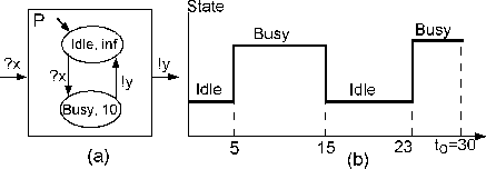
Conventionally the definition of utilization is the percentage of the working time of a machine compared to its total running time. Let's consider a processor P as shown in Figure 4.2(a) which has two states: Busy, which is defined as working time, and Idle, which is defined as ``running, but not working'' time. Once it receives an input ?x, it processes the input and then generates output !y after 10 time units. Figure 4.2(b) illustrates a state trajectory of the processor terminating at $t_o = 30$ . In this trajectory, the total time span of Busy is (15-5)+(30-23)=17, so utilization of the processor is 56.7%=(17/30)*100, while idle's percentage is 100-56.7=43.3%.

Figure 4.2: State Trajectory of a Processor

We can generalize this concept to more than two states. Let's consider the vending machine introduced in Section 3.1.2. Suppose that we have a state trajectory of the vending machine as shown in Figure 4.3. This state trajectory can be seen as a sequences of piece-wise constant segments. The time it takes to transition between states is assumed to be zero.

Figure 4.3: A State Trajectory of Vending Machine

The time duration of a piece-wise constant segment is defined by $td:S \times \mathbb{N} \rightarrow T$ where $\mathbb{N}$ is a set of natural numbers. This function maps from state $s$ and the order $i \in \mathbb{N}$ of a segment piece to a time span value if the segment piece in the state $s$ , otherwise the value is 0. For example, in the state trajectory of Figure 4.3, $td(\verb''Idle'', 1)=5-0=5$ , while $td(\verb''Idle'', 2)=0$ because the state of the second segment is Wait.

Let $C$ be the current state. Then the probability that the current state is $s \in S$ over time from 0 to $t_o$ , denoted by $P(C=s)$ , is

$$P(C=s)= \frac{\underset{i \in N} {\sum} td(s, i)}{t_o}.$$ (5.3)

It is true that

$$\underset{s \in S}{\sum}~\underset{i \in N} {\sum} td(s, i)= t_o.$$ (5.4)

So it is also true that

$$\underset{s \in S}{\sum}P(C=s)=\underset{s \in S}{\sum}\left(\frac{\underset{i \in N} {\sum} td(s, i)}{t_o}\right)= \frac{t_o}{t_o}=1.$$ (5.5)

Example 5.3   Consider the state trajectory of Figure 4.3. Then $P(C=$ Idle) = (5+3+10)/40 = 0.45, $P(C$ =Wait) = (15+5)/40 =0.5, $P(C$ =O_pepsi)=2/40 =0.05, $P(C$ =O_coke)=0. $\square$

Exercise 5.1   Assume that we have a processor as shown in Figure 4.2(a). From the processor, we have an event segment $\omega_{[0,50]}=(?x,10)(!y,20)(?x,35)(!y,45)$ where $(z,t)$ means an event $z$ occurs at $t \in T$ and the observation was performed from 0 to 50. Calculate $P(C$ =Idle) and $P(C$ =Busy) over time [0,50]. $\square$

To calculate $P(C=s)$ , we need to keep track of $\underset{i}{\sum}td(s,i)$ by accumulating all time durations of piece-wise constant time segments when the system is in state $s$ . We will see how to implement this in Section 4.2.2.